Here is your basic one-way and two-way ANOVAs. The assumption check is the same for the one-way or two-way ANOVA, you are looking for an even scattering of dots in all three residual plots and your looking for a straight 45 degree line in the q-q plot. A log transformation often helps with biological data.
Performing repeated measures ANOVAs is a little different and I’ll show that on another post.

#Load data

example<- read.table(url("https://jackrrivers.com/wp-content/uploads/2018/03/example3.txt"), header=T)
example$ID<-as.factor(example$ID)

#One-way
ANOVA<-aov(Dependent~Factor1, data=example)
summary(ANOVA)

#Two-way
ANOVA<-aov(Dependent~Factor1*Factor2, data=example)
summary(ANOVA)

#Checking assumptions 
par(mfrow=c(2,2)) 
plot(ANOVA)

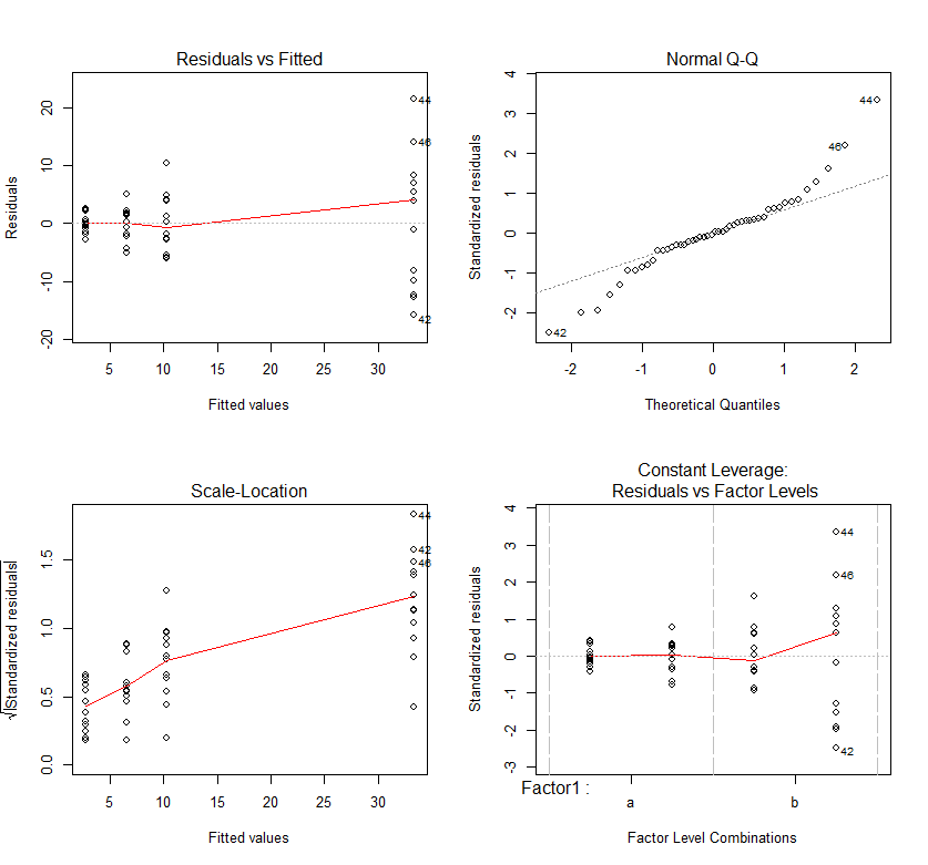
We can see increasing spread in our residual vs fitted plot and standardized residuals vs factor level plot. The sqrt(absolute value of the residuals) are also increasing with predicted value. This means we are breaking the assumption of homoscedasticity.  We also have a lack of normality in our q-q plot. This demonstrates a very common problem in biological data – a proportional relationship between the mean and variance. I.e. groups with larger means also have larger variation. An example of this is that the height of humans vary by cm, while the height of ants vary by 0.01mm. Therefore, variance is not equal – not homoscedastic! The proportional relationship between the mean and the variation can be solved by transforming your data with either a square-root or log transformation (there are others, but try these first). But because you can’t log or square-root a negative value you have to add a fixed value to all the data and this should be just above your most negative value.

#Transformed Two-way
x<-abs(min(example$Dependent))+1

ANOVA<-aov(log(Dependent+x)~Factor1*Factor2, data=example)
summary(ANOVA)

#Checking assumptions 
par(mfrow=c(2,2)) 
plot(ANOVA)

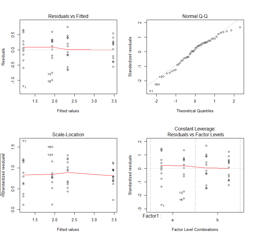
Pretty good!