When the data is unbalanced or there are missing values, repeated measures ANOVAs fail to report unbiased results. Furthermore, all the data of one individual will be ignored if data from one time point is missing. Multi-level linear models gets around this by comparing models of the data, not the data itself, using log-likelihood/Chi squared distribution analyses. Multi-level linear models also avoid sphericity issues. In general multi-level linear models are better in every way to a repeated measures ANVOA.

#Loading data

example<- read.table(url("https://jackauty.com/wp-content/uploads/2023/11/example4.txt"), header=T)
example$ID<-as.factor(example$ID)

#Installing packages (but only if you need to install them)
if(!require(MASS)) install.packages("MASS")
if(!require(sjPlot)) install.packages("sjPlot")
if(!require(ggplot2)) install.packages("ggplot2")
if(!require(emmeans)) install.packages("emmeans")
if(!require(viridis)) install.packages("viridis")


library(ggplot2); library(sjPlot); library(MASS); library(emmeans);

#Running multi-level linear model 

install.packages("lme4")
require(lme4)

lme1<-lmer(Dependent~1 + (1|ID), data=example, na.action=na.omit)
lme2<-update(lme1, .~. +Factor1)
lme3<-update(lme2, .~. +Factor2)
lme4<-update(lme3, .~. +Factor1*Factor2)

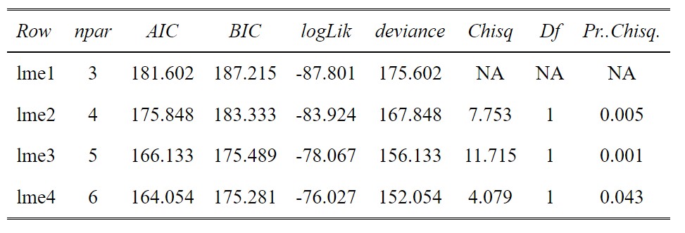
anova(lme1,lme2,lme3,lme4)

Assumption checking

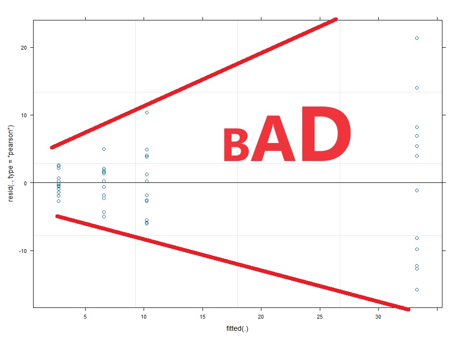
Now with multi-level linear models (AKA repeated measures ANOVA) there are two kinds of residuals. There is the variability of the raw data around the predicted value (this is the conditional residual), and the variability of the random effect (e.g. animal or human). The random effects should be normalish but don’t have to be homoscedastic. The conditional residuals should be both normal and homoscedastic.

#Assumption check of conditional residuals
plot(lme4)

#Now we check for normality of the conditional  residuals
qqnorm(resid(lme4))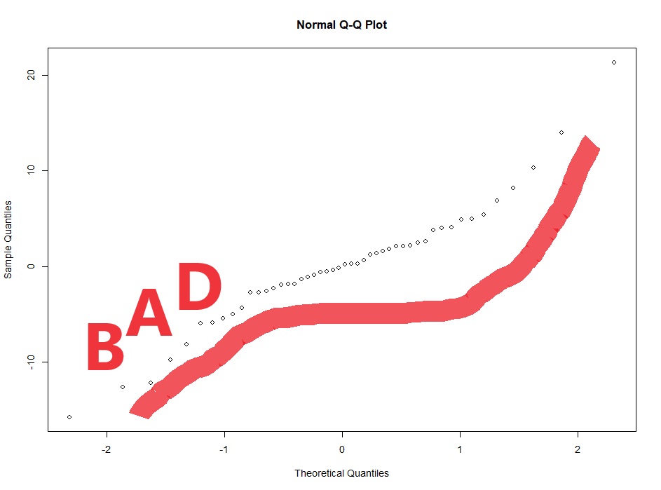

# checking the normality of the random effects (here random intercept):
qqnorm(ranef(lme4)$ID$'(Intercept)', 
       main="Q-Q plot for the random intercept")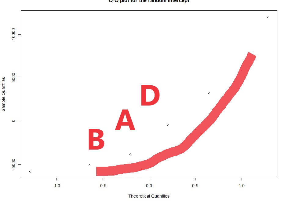

Transforming the data

So you can just have a guess at a transformation needed. The wedge shaped residual vs fitted plot above tells us we need a shrinking transformation like a LOG10 or square root. However, if we can take the researcher out of the process this is better. What if the LOG10 and square root have similar diagnostic plots, but the LOG10 gives you significant results and the square root transformation gives you p=0.051. You might be tempted to choose the LOG10 transformation because it gives you significance.

What we can do is a BoxCox transformation. This is an automated process that transforms your data by a range of powers and evaluates the normality of the residuals. Then it chooses the power (Selected.lamda) that produces the most normally distributed residuals. Typically, when you solve normality, you also solve homoscedasticity.

Now you can do this on a multi-level linear model, but often fixing a simple model will also fix the complex model. So we’ll run a simple linear model, calculate what we should transform the data by, then apply that transformation to our multi-level linear model.

#Making the simple linear model
simple.linear<-lm(Dependent~Factor1*Factor2, data=example)

#BoxCox transformation 
boxcox<-boxcox(simple.linear,lambda = seq(-5, 5, 1/1000), plotit = TRUE ) 

Selected.lambda <-boxcox$x[boxcox$y==max(boxcox$y)] 
Selected.lambda 

#Run the transformed model 
lme1<-lmer((Dependent+1)^Selected.lambda~1 + (1|ID), data=example, na.action=na.omit)
lme2<-update(lme1, .~. +Factor1)
lme3<-update(lme2, .~. +Factor2)
lme4<-update(lme3, .~. +Factor1*Factor2)

anova(lme1,lme2,lme3,lme4)

#Assumption check
plot(lme4)
qqnorm(resid(lme4))

# checking the normality of the random effects (here random intercept):
qqnorm(ranef(lme4)$ID$'(Intercept)', 
       main="Q-Q plot for the random intercept")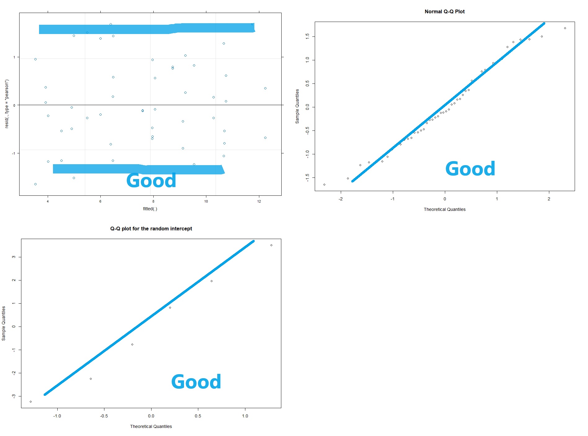

Posthocs!

OK this is a Post-hoc analysis with a priori selected comparisons. Perhaps we don’t want to do all the comparisons, because some are useless. For example, why compare Females on Drug with Males on Placebo? That doesn’t make sense. So in this, we select our comparisons and adjust for only those comparisons.

#Posthoc/Planned contrasts 
post <- emmeans(lme4, pairwise ~ Factor1*Factor2, adjust="none") 

posthoc<-summary(post) 

#Look at the table of potential comparisons
tab_df(posthoc$contrasts[,c(1,4)],show.rownames =T)  

#Select the comparison you are interested in but adding the row numbers below
comparisons<-c(1,2,5,6)

#Build a dataframe of all the comparisons (contrasts) and the unadjusted p values
p.value<-data.frame(cbind(posthoc$contrasts["contrast"],posthoc$contrasts["p.value"]))

ptable<-p.value[comparisons,]

#Create a column of adjusted p values using the Holm-Sidak method
ptable$padj<-p.adjust(ptable$p.value, method="holm") 

#View the table in a pretty way
tab_df(ptable,digits = 4)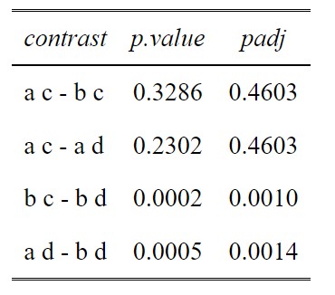  

How I would publish the above method.

Linear mixed modelling was used to evaluate the effect of explanatory variables on the dependent variable (package lme4, Bates et al. 2015). All factors and interactions were modelled as fixed effects. A within-subject design with random intercepts were used for all models. The significance of inclusion of an independent variable or interaction terms were evaluated using log-likelihood ratio. Holm-Sidak post-hocs were then performed for pair-wise comparisons using the least square means (package “emmeans”, Lenth 2023). Homoskedasticity and normality of the Pearson residuals were evaluated graphically using predicted vs residual and Q-Q plots, respectively, and Box Cox transformations were applied when necessary (package “MASS” Venables 2002). All analyses were performed using R (version 4.3.3).

#Making a reference list 
pkg <- c("MASS","sjPlot","lme4","emmeans") 

#Create a loop to build a dataframe of the references
citation_list<-factor() 

for(i in pkg){   citation_list<- c(citation_list,paste(capture.output(print(citation(i), style ="text",bibtext=F)), collapse="\n")) }

#Display the dataframe nicely with sjPlot's tab_df
tab_df(   data.frame(citation_list), col.header="References", sep=" ") 

Venables WN, Ripley BD (2002). _Modern Applied Statistics with S_, Fourth edition. Springer, New York. ISBN 0-387-95457-0, .

Lüdecke D (2023). _sjPlot: Data Visualization for Statistics in Social Science_. R package version 2.8.14, .

Wickham H (2016). _ggplot2: Elegant Graphics for Data Analysis_. Springer-Verlag New York. ISBN 978-3-319-24277-4, .

Lenth R (2023). _emmeans: Estimated Marginal Means, aka Least-Squares Means_. R package version 1.8.6, .

Bates D, Mächler M, Bolker B, Walker S (2015). “Fitting Linear Mixed-Effects Models Using lme4.” _Journal of Statistical Software_, *67*(1), 1-48. doi:10.18637/jss.v067.i01 .

All the code at once! (easier to copy)

#Installing packages (but only if you need to install them)

if(!require(MASS)) install.packages("MASS")
if(!require(sjPlot)) install.packages("sjPlot")
if(!require(ggplot2)) install.packages("ggplot2")
if(!require(emmeans)) install.packages("emmeans")
if(!require(viridis)) install.packages("viridis")


library(ggplot2); library(sjPlot); library(MASS); library(emmeans);

#Loading data

example<- read.table(url("https://jackauty.com/wp-content/uploads/2023/11/example4.txt"), header=T)
example$ID<-as.factor(example$ID)


#Running multi-level linear model 
lme1<-lmer(Dependent~1 + (1|ID), data=example, na.action=na.omit)
lme2<-update(lme1, .~. +Factor1)
lme3<-update(lme2, .~. +Factor2)
lme4<-update(lme3, .~. +Factor1*Factor2)

anova(lme1,lme2,lme3,lme4)
#Assumption check
plot(lme4)
qqnorm(resid(lme4))

# checking the normality of the random effects (here random intercept):
qqnorm(ranef(lme4)$ID$'(Intercept)', 
       main="Q-Q plot for the random intercept")

simple.linear<-lm(Dependent~Factor1*Factor2, data=example)

#BoxCox transformation 
boxcox<-boxcox(simple.linear,lambda = seq(-5, 5, 1/1000), plotit = TRUE ) 

Selected.lambda <-boxcox$x[boxcox$y==max(boxcox$y)] 
Selected.lambda 

#Run the transformed model 
lme1<-lmer((Dependent+1)^Selected.lambda~1 + (1|ID), data=example, na.action=na.omit)
lme2<-update(lme1, .~. +Factor1)
lme3<-update(lme2, .~. +Factor2)
lme4<-update(lme3, .~. +Factor1*Factor2)

tab_df(anova(lme1,lme2,lme3,lme4),show.rownames =T, digits=3)

#Assumption check
plot(lme4)
qqnorm(resid(lme4))

# checking the normality of the random effects (here random intercept):
qqnorm(ranef(lme4)$ID$'(Intercept)', 
       main="Q-Q plot for the random intercept")

#Create a linear model and do a Box-Cox transformation


#Posthoc/Planned contrasts
#Posthoc/Planned contrasts 
post <- emmeans(lme4, pairwise ~ Factor1*Factor2, adjust="none") 

posthoc<-summary(post) 

tab_df(posthoc$contrasts[,c(1,4)],show.rownames =T)  

##Now select the rows of the comparisons you are interested in

comparisons<-c(1,2,4)

#Build a dataframe of all the comparisons (contrasts) and the unadjusted p values
p.value<-data.frame(cbind(posthoc$contrasts["contrast"],posthoc$contrasts["p.value"]))

#Select the comparison you are interested in
comparisons<-c(1,2,5,6)
ptable<-p.value[comparisons,]

#Create a column of adjusted p values using the Holm-Sidak method
ptable$padj<-p.adjust(ptable$p.value, method="holm") 

#View the table in a pretty way
tab_df(ptable,digits = 4)  

#Making a reference list 
pkg <- c("MASS","sjPlot","lme4","emmeans") 

#Create a loop to build a dataframe of the references
citation_list<-factor() 

for(i in pkg){   citation_list<- c(citation_list,paste(capture.output(print(citation(i), style ="text",bibtext=F)), collapse="\n")) }

#Display the dataframe nicely with sjPlot's tab_df
tab_df(   data.frame(citation_list), col.header="References", sep=" ")