Generalized mixed modelling
Sometimes you know your data can’t follow a normal distribution even after transformation – such as count data or yes/no data. If this is the case, then generalized mixed modelling is the way to go. Basically it’s very similar to general linear modelling which assumes normality of the population distribution, but instead it assumes a different underlying distribution (and it models using maximum likelihood, not minimizing the residuals). For this analysis we have count data (the number of neutrophils in the brain) and a random effect of siblings. Siblings is treated as a random effect because with experiments involving large numbers that come from one parent pair (like fish or fly data), we tend to think that the siblings aren’t independent and perhaps the parents are effecting the outcome. Therefore, we model this lack of independence by treating siblings as a random effect. In fish data we call a bunch of siblings a “clutch”.
To do the analysis, first select the best model. For count data Poisson is the obvious choice, but there are several potential link functions (similar to transformations). So we must select the optimal link function for the Poisson model. However, Poisson has the assumption that the mean is equal to the variance. This is true if each count is completely independent, like counting cars on a quiet country road. However, in biology this is often not the case, in this example having one neutrophil increases your chances of having two neutrophils because an inflammatory response is happening. This is more like a busy road where one car driving by increases the chances of a second car driving by (is it rush hour?), the counts aren’t independent. In this case a negative binomial is a good family to model the data. It has two parameterization methods (the method by which it predicts the lack of independence of the counts). So now you have to model the Poisson models with the three link functions and the negative binomial model with the two parameterization methods and then see which is best. For this we use the Akaike Information Criteria (AIC). With AIC the lower the better, so we will select the model with the lowest AIC.
#Packages
require("lme4")
require("ggplot2")
require("glmmADMB")
require("car")
require("fitdistrplus")

#Loading data example.count<- read.table(url("https://jackauty.com/wp-content/uploads/2018/10/count.txt"), header=T) str(example.count) #Generalized mixed modelling try(glmm.a<-glmmadmb(Neutrophils~Factor1+ (1|Clutch), data=example.count,family="nbinom")) try(glmm.b<-glmmadmb(Neutrophils~Factor1+ (1|Clutch), data=example.count,family="nbinom1")) try(glmm.c<-glmer(Neutrophils~Factor1+ (1|Clutch), data=example.count, family=poisson(link="log"))) try(glmm.d<-glmer(Neutrophils~Factor1+ (1|Clutch), data=example.count, family=poisson(link="identity"))) try(glmm.e<-glmer(Neutrophils~Factor1+ (1|Clutch), data=example.count,family=poisson(link="sqrt"))) AIC(glmm.a,glmm.b,glmm.c,glmm.d,glmm.e) df AIC glmm.a 4 270.5040 glmm.b 4 273.9180 glmm.c 3 446.7101 glmm.d 3 475.2077 glmm.e 3 461.6097
From this we can see that the negative binomial model is much better and the “nbinom” parameterization is preferred. Now we can continue with our analysis very much like a normal multi-level linear model.
#Build model with and without our independent variable (Factor1)
glmm1<-glmmadmb(Neutrophils~1 + (1|Clutch), data=example.count,family="nbinom")
glmm2<-update(glmm1, .~. +Factor1)
anova(glmm1,glmm2)
Analysis of Deviance Table

Model 1: Neutrophils ~ 1
Model 2: Neutrophils ~ +Factor1
 NoPar LogLik Df Deviance Pr(>Chi)
1 3 -134.27
2 4 -131.25 1 6.028 0.01408 *
---
Our factor significantly improves the model! From this we might say in our publication – “There was a significant effect of factor on neutrophil count (χ2(1)=6.028, p=0.014).”. But first! We have to check the assumptions, this is a little bit different to multi-level linear modelling.
- Is the data approximately distributed appropriately (negative binomial)?
- Are there outlying data points?
- Are the residuals centered around zero for each factor?
- Is there zero inflation (more zeros than expected, this is common in biological data)?
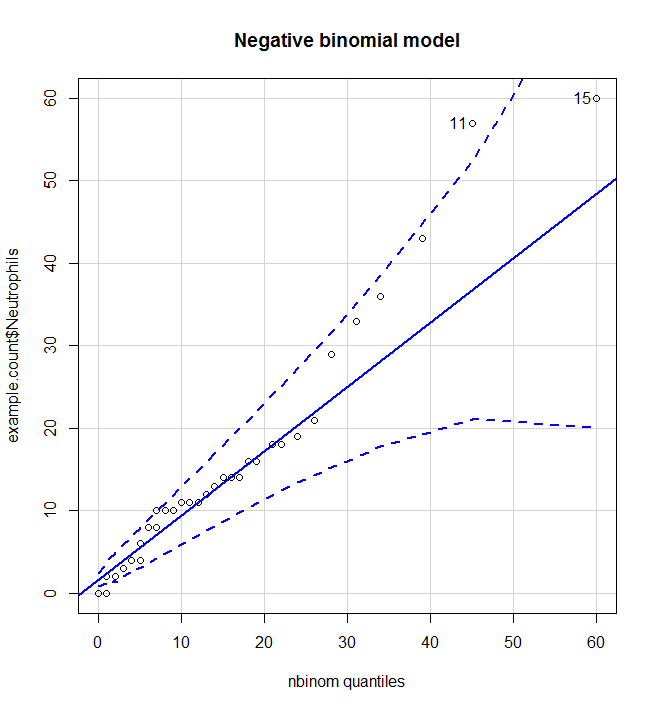
Is the data approximately distributed appropriately (negative binomial)?
From this we can see that the negative binomial model is much better than the Poisson model and most data points lie between the 95% CI of the expected distribution.
#Is the data approximately distributed appropriately (negative binomial)? poisson <- fitdistr(example.count$Neutrophils, "Poisson") qqp(example.count$Neutrophils, "pois", lambda=poisson$estimate, main="Poisson model")nbinom<-fitdistr(example.count$Neutrophils, "negative binomial") qqp(example.count$Neutrophils, "nbinom", size=nbinom$estimate[[1]], mu=nbinom$estimate[[2]], main="Negative binomial model")
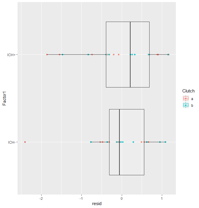
Are there outlying data points? AND Are the residuals centered around zero for each factor?
Plotting the residuals against Factor we can see if the model fitted sensible coefficients and if there are outlying data points. Here we are looking to see if the residuals cluster around zero and that there are no extreme residuals.
Here we can see that the residuals around both factor levels are centered around zero. The random effect of “clutch” seems to model well, with no clustering. There is one residual with an absolute value greater than two. This is slightly concerning with a data set this small. It could be worth checking your lab notes for anything peculiar. I don’t tend to remove data points without a practical reason, for example I might read in my lab notes that this zebra fish looked a lot like a mouse, then I would remove it.
#Are there outlying data points? AND Are the residuals centered around zero for each factor?
augDat <- data.frame(example.count,resid=residuals(glmm2,type="pearson"),
 fitted=fitted(glmm2))
ggplot(augDat,aes(x=Factor1,y=resid,col=Clutch))+geom_point()+geom_boxplot(aes(group=Factor1),alpha = 0.1)+coord_flip()
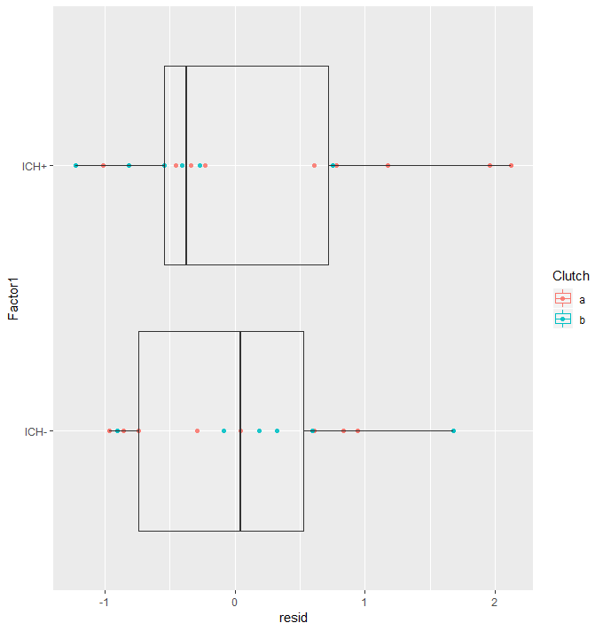
Is there zero inflation (more zeros than expected, this is common in biological data)?
Here we run the same model but with zeroInflation=T, then we check the AIC and find that the zero-inflation model is better! This sucks because now we have to run the whole thing again with zeroInflation=T. On the re-run, the p-value “improved” and outliers were gone, showing that they were due to zero inflation (and not my zebra fish being a mouse)! So I guess it all works out in the end.
#Is there zero inflation
try(glmm.zero<-glmmadmb(Neutrophils~Factor1+ (1|Clutch), data=example.count,family="nbinom", zeroInflation = T))
AIC(glmm.zero,glmm2)

          df AIC
glmm.zero  5 268.298
glmm2      4 270.504

#Quick rerun
glmm1.zero<-glmmadmb(round(Neutrophils)~1 + (1|Clutch), data=example.count,family="nbinom", zeroInflation = T)
glmm2.zero<-update(glmm1.zero, .~. +Factor1)
anova(glmm1.zero,glmm2.zero)

Analysis of Deviance Table
Model 1: round(Neutrophils) ~ 1
Model 2: round(Neutrophils) ~ +Factor1
 NoPar LogLik Df Deviance Pr(>Chi)
   4  -134.14
   5  -129.15  1  9.976   0.001586 **

#Quick assumption check
#Are there outlying data points? AND Are the residuals centered around zero for each factor?
augDat <- data.frame(data,resid=residuals(glmm2,type="pearson"),
 fitted=fitted(glmm2))
ggplot(augDat,aes(x=Factor1,y=resid,col=Clutch))+geom_point()+geom_boxplot(aes(group=Factor1),alpha = 0.1)+coord_flip()
Publication methods:
For discrete data and data with non-normal distributions, generalized linear mixed modelling was used (GLMM) (lme4, Douglas et al. 2015; glmmADMB Fournier et al. 2012 & Skaug et al. 2016). Again “Clutch” was treated as a random effect modelled with random intercepts for all models. Appropriate families were selected based on the data distribution. Numerous families and link functions were evaluated where necessary and the optimal parameters were selected based on the Akaike information criterion (AIC). For mobile or non-mobile (yes/no) data a logistic regression was used, for count data (number of cells) a negative binomial family was selected. The significance of inclusion of an independent variable or interaction terms were evaluated using log-likelihood ratio. Holm-Sidak post-hocs were then performed for pair-wise comparisons using the least square means (LSmeans, Russel 2016). Pearson residuals were evaluated graphically using predicted vs level plots. All analyses were performed using R (version 3.5.1, R Core Team, 2018).
Douglas Bates, Martin Maechler, Ben Bolker, Steve Walker (2015). Fitting Linear Mixed-Effects Models Using lme4. Journal of Statistical Software, 67(1), 1-48.<doi:10.18637/jss.v067.i01>.
Russell V. Lenth (2016). Least-Squares Means: The R Package lsmeans. Journal of Statistical Software, 69(1), 1-33.<doi:10.18637/jss.v069.i01>
Fournier DA, Skaug HJ, Ancheta J, Ianelli J, Magnusson A, Maunder M, Nielsen A, Sibert J (2012). “AD Model Builder: using automatic differentiation for statistical inference of highly parameterized complex nonlinear models.” _Optim. Methods Softw._, *27*, 233-249.
Skaug H, Fournier D, Bolker B, Magnusson A, Nielsen A (2016). _Generalized Linear Mixed Models using ‘AD Model Builder’_. R package version 0.8.3.3.
R Core Team (2018). R: A language and environment for statistical computing. R Foundation for Statistical Computing, Vienna, Austria. URL https://www.R-project.org/.